As I mentioned in my previous post about this project’s background, when children turn three, they transition from receiving services under IDEA Part C to IDEA Part B (Early Childhood Technical Assistance Center, 2024). Infants and toddlers exit Early Intervention (EI) services for various reasons, and significant disparities exist in how children from different racial backgrounds experience this transition.
The odds ratio analysis measures how much more or less likely an outcome is for one group compared to another (Hosmer et al., 2013). However, if not used mindfully, the results can be too simplistic and may end up reinforcing common narratives that unfairly blame certain groups for disparities. This kind of oversimplification ignores the complexity of intersectionality (Crenshaw, 1989) that marginalized communities live. It’s also worth noting that Karl Pearson, who created the chi-square test, is believed to have developed statistical tools to support eugenics (Castillo & Strunk, 2025, p. 3).
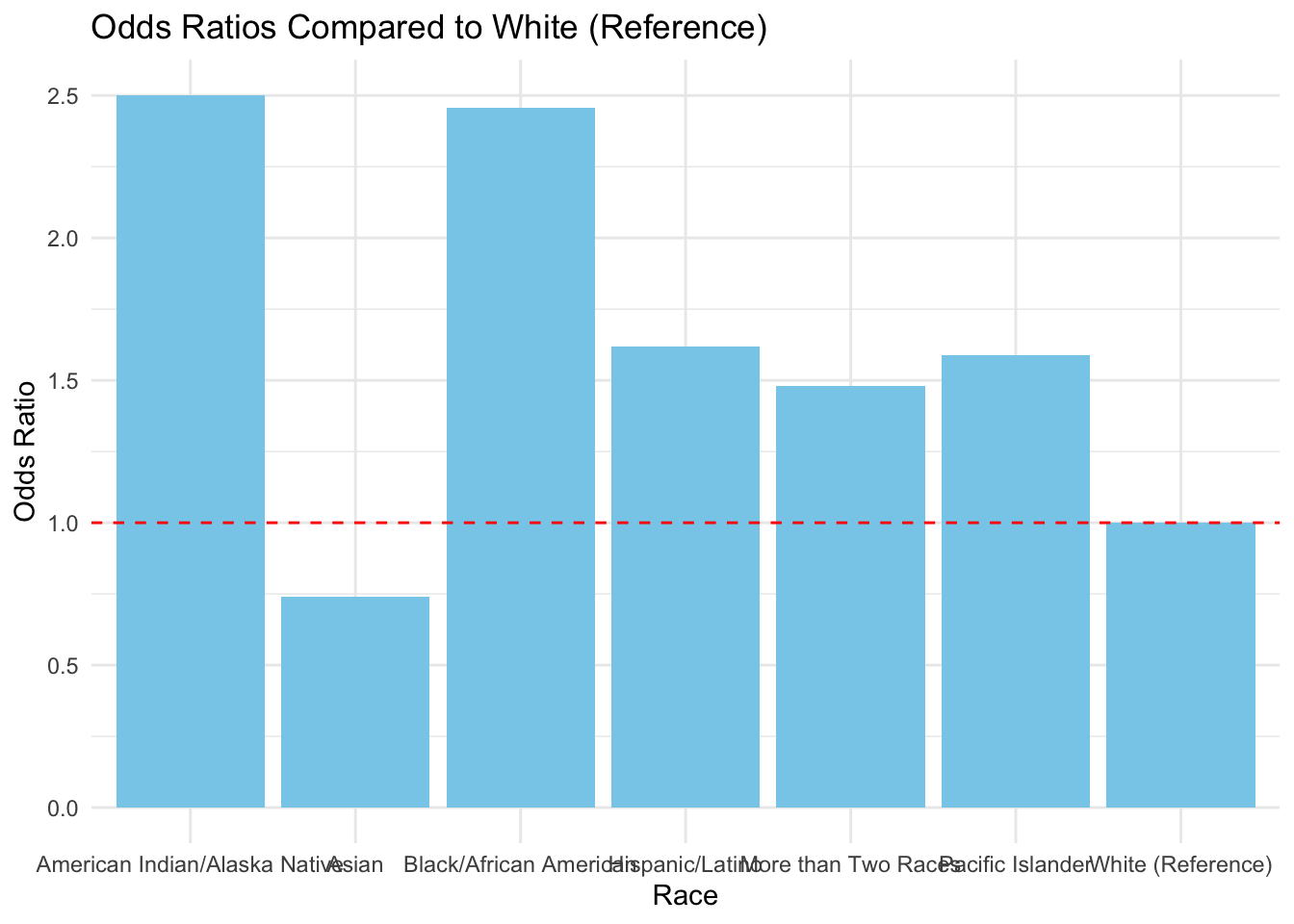
First, I ran an odds ratio analysis for the “Dismissed” exit category across all racial groups. Then, I tried creating bar charts to visualize the results.
Code
ggplot(or_us_white, aes(x =factor(group, levels =sort(unique(group))), y = odds_ratio)) +geom_col(fill ="skyblue") +geom_hline(yintercept =1, linetype ="dashed", color ="red") +labs(title ="Odds Ratios Compared to White (Reference)", x ="Race", y ="Odds Ratio") +theme_minimal()
Code
# with flipped coordinatesggplot(or_us_white, aes(x =factor( group, levels =sort(unique(group))), y = odds_ratio)) +geom_col(fill ="skyblue") +geom_hline(yintercept =1, linetype ="dashed", color ="red") +coord_flip() +labs(title ="Odds Ratios Compared to White (Reference)", x ="Group", y ="Odds Ratio" ) +theme_minimal()
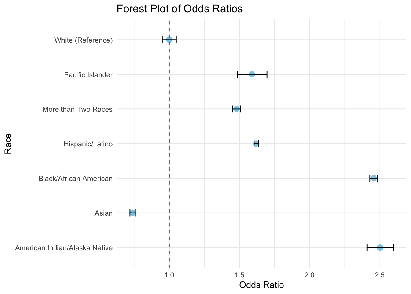
However, using a forest plot for odds ratio has traditionally been considered appropriate, because they can show confidence intervals, making it easier to understand the precision of each estimate. To create a forest plot, we need to prepare a table that includes not only the odds ratios but also the confidence intervals for each comparison.
Here, I used geom_errorbar() from ggplot().
Code
ggplot(or_us_white_ci, aes(x = group, y = odds_ratio)) +geom_point(size =3, color ="skyblue") +geom_errorbar(aes(ymin = ci_lower, ymax = ci_upper), width =0.2) +geom_hline(yintercept =1, linetype ="dashed", color ="red") +coord_flip() +labs(title ="Forest Plot of Odds Ratios",x ="Race",y ="Odds Ratio" ) +theme_minimal()
Then, I reversed the alphabetical order of the Y-axis.
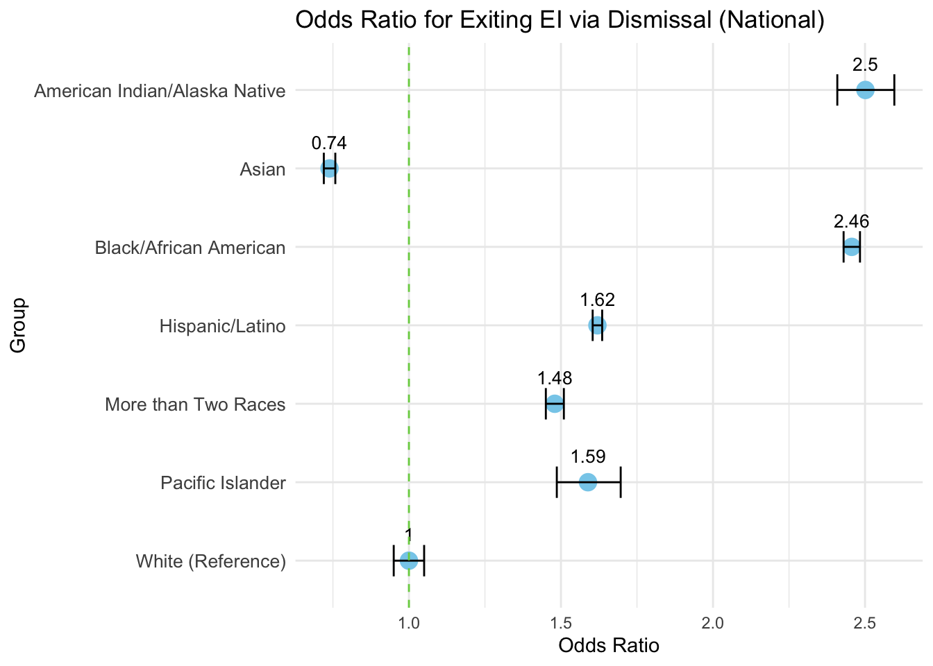
Finally, I made the following adjustments to make the chart easier to read:
Increased the size of the blue dots
Made the the X-axis labels larger
Added data labels above the dots.
Do you see how the odds ratios highlight the over- and under-representations in the “Dismissed” category? (Just a reminder, this category represents cases where agencies “lose contact” with families, leading to disqualification.)
Code
ggplot(or_us_white_ci, aes(x = group, y = odds_ratio)) +geom_point(size =4, color ="skyblue") +geom_errorbar(aes(ymin = ci_lower, ymax = ci_upper), width =0.4) +geom_text(aes(label =round(odds_ratio, 2)), vjust =-1.5, size =3.5) +geom_hline(yintercept =1, linetype ="dashed", color ="#7ad151") +coord_flip() +labs(title ="Odds Ratio for Exiting EI via Dismissal (National)",x ="Group",y ="Odds Ratio" ) +theme_minimal() +theme(axis.text.y =element_text(size =10) )
For my dissertation, I plan to re-analyze the same datasets by comparing each group to the overall category average across all races. This way, I can avoid using White children and families as the norm for comparison.
I will also examine how infants and toddlers from different racial groups are represented in Early Intervention (EI) compared to census data. I will then conduct chi-square analyses with adjusted standardized residuals to explore exit patterns based on children’s home language(s) and Medicaid eligibility in Oregon. Additionally, a comprehensive literature review incorporating both quantitative and qualitative studies will help amplify the voices of the families.
Thank you for reading, and please stay connected through my LinkedIn page!